SECTION 1 Data
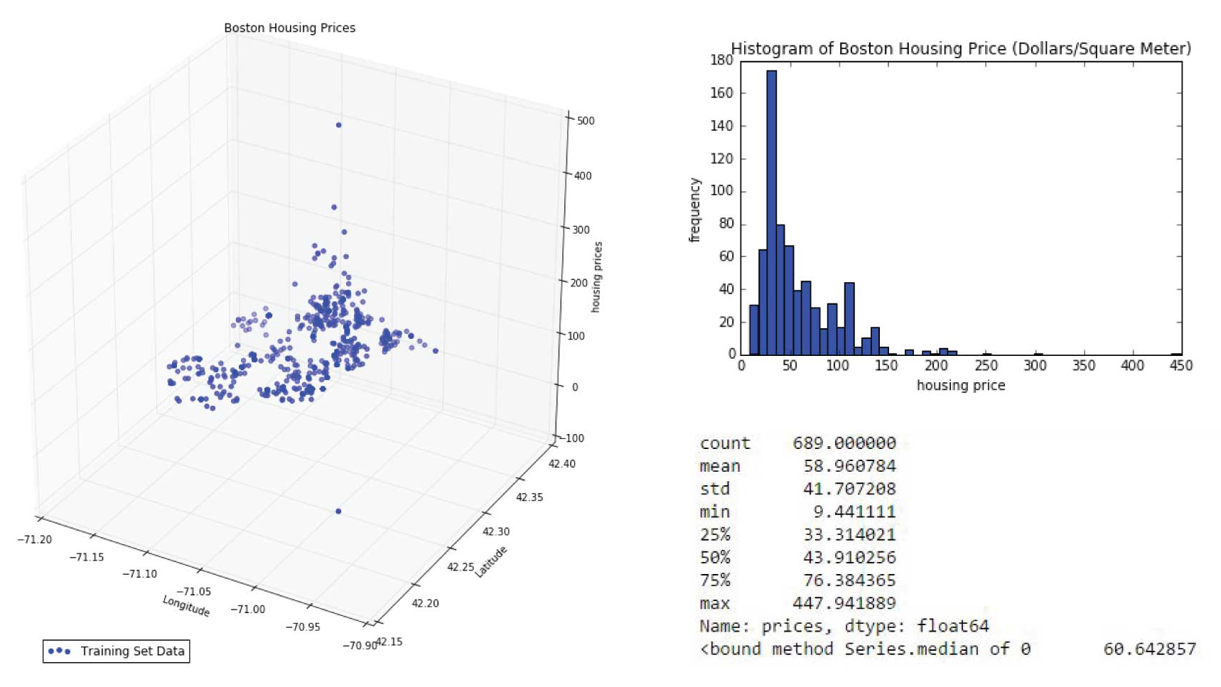
The basic stats of housing price in the city of Boston
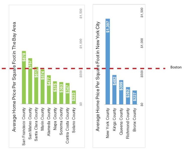
We explored housing prices statistics and the relationshpi between Boston housing price and our dataset features. Boston's average housing price is around $58/m2 and the median is about $60/m2 while it has a range from $9.4/m2 to $447/m2, which ranks quite high nationally.According to Zillow home values report , the national average housin gprice is $13.2/m2.(http://www.zillow.com/home-values/)
3 0
SECTION 2 Prediction Models
What features depict boston housing price?
The Baseline Model
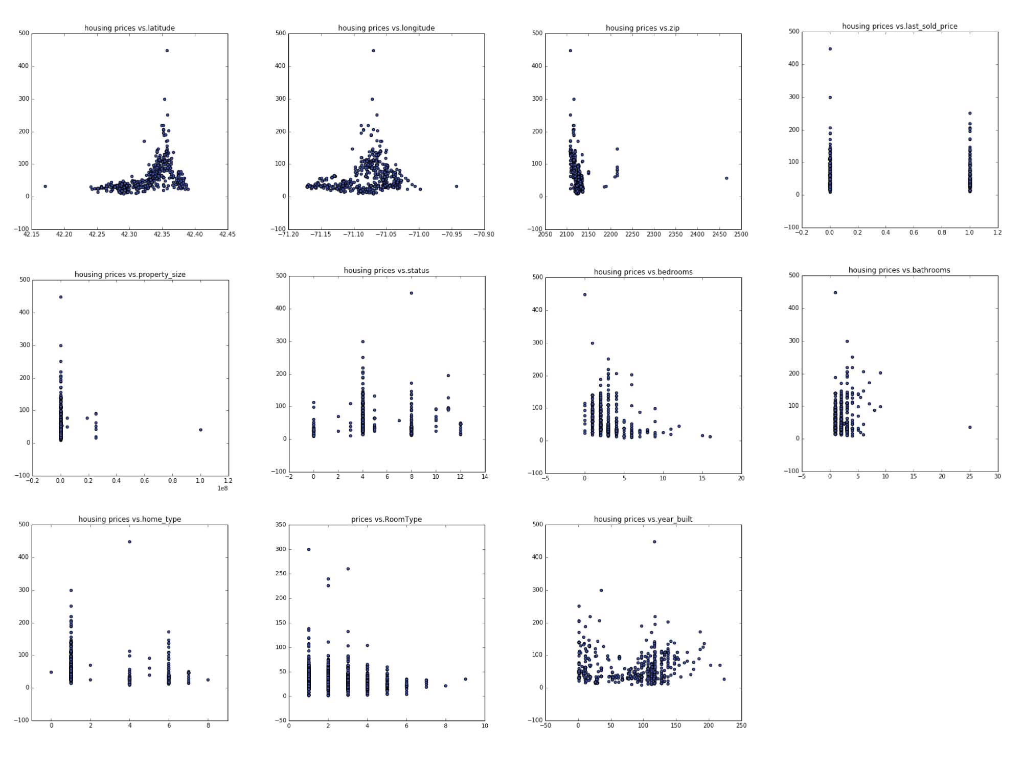
Zillow Features (used for baseline model):
Longitude,Latitude,Zipcode,SoldOnce(bool),Bedrooms,Bathrooms,House type,land size
These features come with the data set we obtained from Zillow websites. A simple linear regression of housing price with these features gives a prediction with test score (R2) of 0.3 which is not optimal as we can see that we are missing a lot of determinant features to price of a house such as wether it has garage, central heating, or if it is newly renovated.
The Baseline Model
The baseline model involves features only from Zillow resource. There are 727 houses data in total, and we had to filling in missing 327 land size and 55 missing building age values through KNN methods using the location, and house type features to estimate. The result of the baseline model is not so predicative with an measure around 0.32 in R square of the test set.
base=['longitude', 'latitude',
       'bathrooms', 'last_sold_price', 'property_size', 'zip', 'status',
       'bedrooms', 'year_built', 'home_type']
xlinear = data[base].values
n = xlinear.shape[0]
n_train = int(np.round(n * 0.4))

# First 40% train, remaining test
xlinear_train = xlinear[:n_train, :]
y_train = y[:n_train]
xlinear_test = xlinear[n_train:, :]
y_test = y[n_train:]
reg = Lin_Reg() #automatically fits intercept (adds column of one's) for you
reg.fit(xlinear_train, y_train)
ylinearpred = reg.predict(xlinear_test)
train_r_squared_plain = reg.score(xlinear_train, y_train)
test_r_squared_plain = reg.score(xlinear_test, y_test)
Plain Regression: R^2 score on training set 0.316326357898
Plain Regression: R^2 score on test set 0.390477980533
[ -8.86686784e+01 4.34318178e+02 3.10418622e+00 -6.93186846e+00
-9.17424434e-07 -2.87754641e-01 2.54193714e+00 -3.32795469e+00
-2.75095526e-03 -4.95002385e+00]

The Improved Model
To imporve the model, first we would add datas that we obtained from google places, boston city government site and google street views.
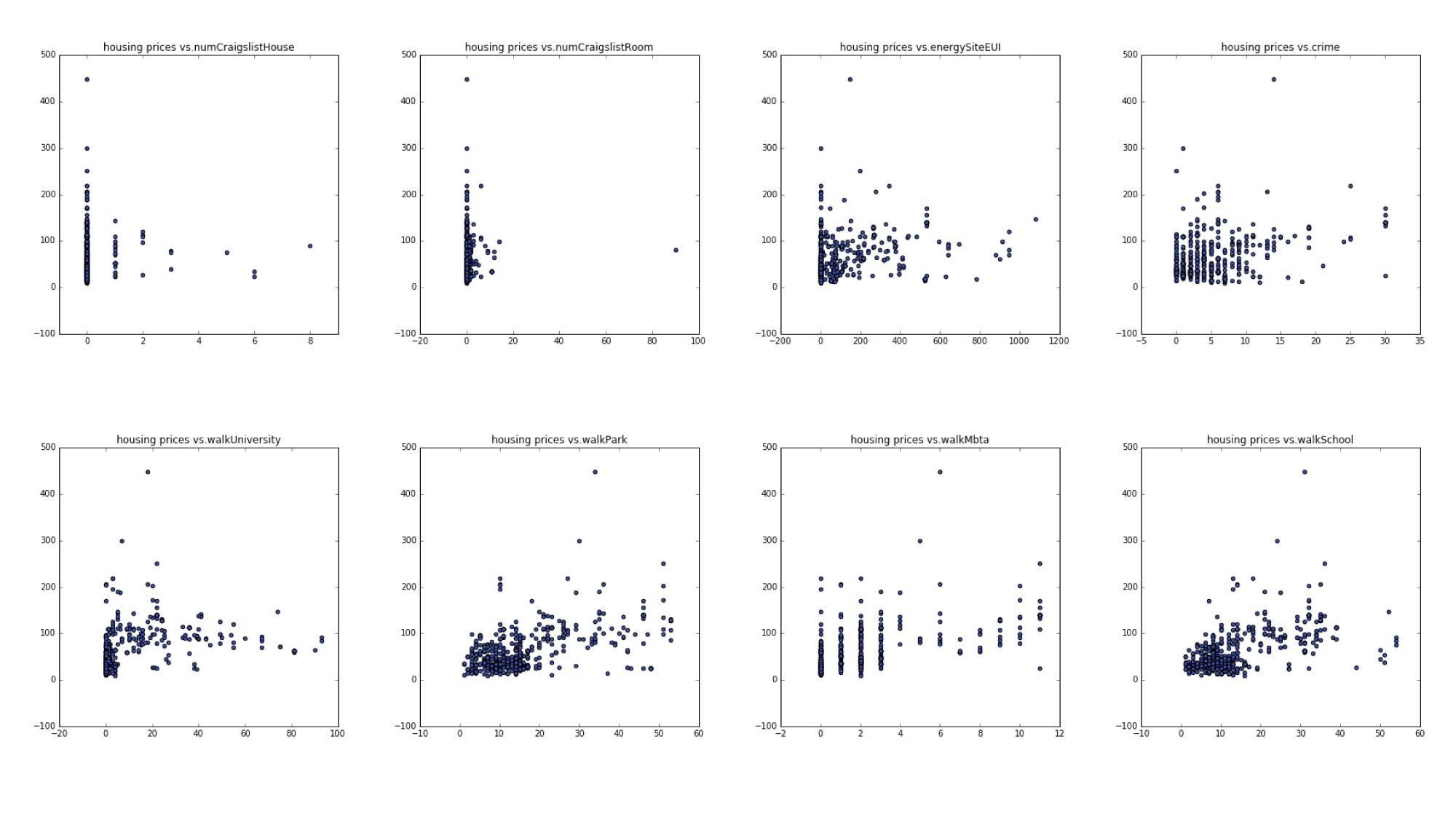
City Infrastructural Features:
These include:
walking distance to mbta, walking distance to school(k-12 education),walking distance to university, walking distance to park, crime rates, land energy use, craiglist house posting, craiglist room posting
These factors appear to be crucial prediction features, especially in a cultural city with strong academic resources like Boston, school districts appeared to be a major factor.
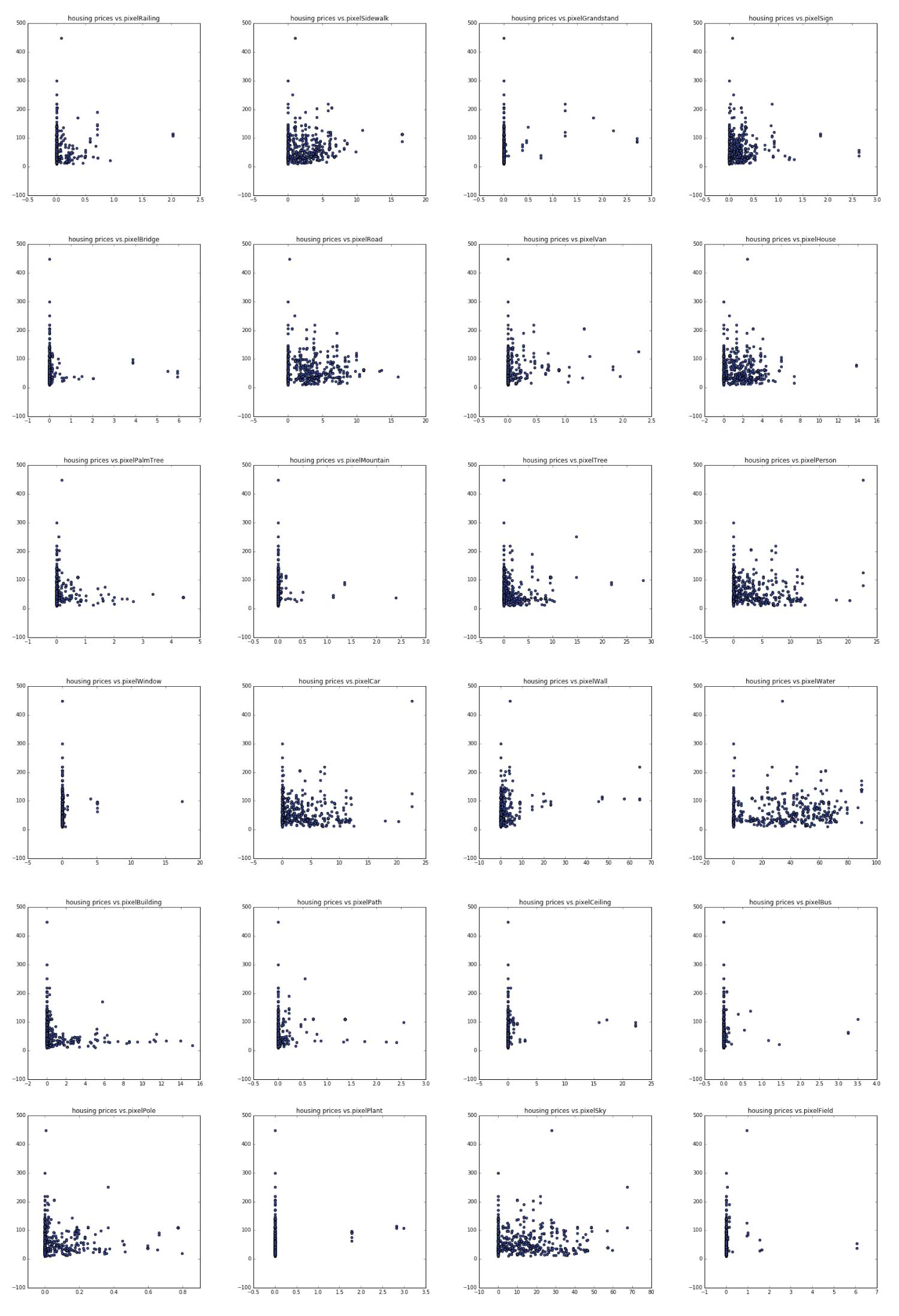
Google Street views data would capture interesitng charachteristics of the neighborhoods and we plot prices in relationship with features deployed from the streetview images. Among these some interesting ones are pixelWater, pixelVan, pixelCar,pixel road, pixelSidewalk, pixelSky. These somewhat shows correlation with housing price.
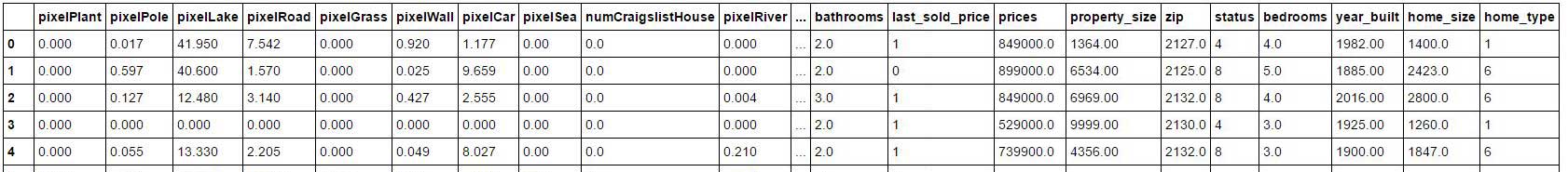
The combination of zillow data set and these features that we gathered from other sources have 40 features together, and it looks like this after processing:
Forward and Backward selection of these features picked 'pixelWall' 'pixelCeiling' 'pixelPath' 'walkSchool' 'walkMbta' 'energySiteEUI' 'walkPark' 'pixelBridge' 'pixelWindow' 'pixelGrandstand' 'latitude' 'bathrooms' 'bedrooms' while pixel window is the only different feature from the two selections.
Step-wise forward subset selection: [3, 8, 9, 12, 13, 14, 18, 25, 29, 30, 34, 35, 40] ['pixelWall' 'pixelCeiling' 'pixelPath' 'walkSchool' 'walkMbta' 'energySiteEUI' 'walkPark' 'pixelBridge' 'pixelWindow' 'pixelGrandstand' 'latitude' 'bathrooms' 'bedrooms']
Step-wise backward subset selection: [3, 8, 9, 12, 13, 14, 18, 25, 30, 34, 35, 40] ['pixelWall' 'pixelCeiling' 'pixelPath' 'walkSchool' 'walkMbta' 'energySiteEUI' 'walkPark' 'pixelBridge' 'pixelGrandstand' 'latitude' 'bathrooms' 'bedrooms']
Using these selected features, a linear regression model now have a much prediction power as the R square meausre increased to around 0.55reg = Lin_Reg() #automatically fits intercept (adds column of one's) for you reg.fit(xlinear_train, y_train) ylinearpred = reg.predict(xlinear_test) train_r_squared_plain = reg.score(xlinear_train, y_train) test_r_squared_plain = reg.score(xlinear_test, y_test) print 'Plain Regression: R^2 score on training set', train_r_squared_plain print 'Plain Regression: R^2 score on test set', test_r_squared_plain print backward print reg.coef_
Plain Regression: R^2 score on training set 0.554806605344
Plain Regression: R^2 score on test set 0.552280768531
['pixelWall' 'pixelCeiling' 'pixelPath' 'walkSchool' 'walkMbta'
'energySiteEUI' 'walkPark' 'pixelBridge' 'pixelGrandstand' 'latitude'
'bathrooms' 'bedrooms']
[ 1.66975864e+00 -5.08047923e+00 1.02931553e+01 8.37755472e-01
-4.70824163e-01 -2.65410930e-03 9.89936107e-01 -9.55759953e+00
4.06865061e+01 3.34295897e+02 2.07474792e+00 -4.47986540e+00]

Visulization of the original data set and its predicted value:
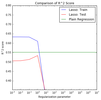
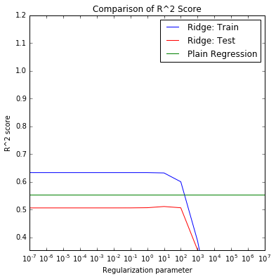
Lasso and ridge models have similiar (slightly smaller) R square compared to the linear regression model. They picked up more features thant the backward and forward selection . After tuning alpha parameter, the results are below:
 x_std = Standardize(with_mean=False).fit_transform(x)

# Lasso regression
reg = Lasso_Reg(alpha =1)
reg.fit(x_std, y)
coefficients = reg.coef_

print 'Lasso:'
print 'Coefficients:', coefficients
print  'Predictors with non-zero coefficients:', [i for i, item in enumerate(coefficients) if abs(item) > 0]
print data.columns.values[[i for i, item in enumerate(coefficients) if abs(item) > 0]]
Lasso:
Coefficients: [ 1.78022984 0.76351372 -1.62028417 3.85289307 1.19614439 0. 0.
-0.16021163 -3.09622089 2.86537383 -0.03692707 1.54431305
9.99467568 4.29210187 -1.21071298 0.09701096 0. 1.49519728
6.15427688 0. 0. 0. -0.23433414 0. -0.
-2.08276022 -0. -0. -1.34738636 0.19296128
5.31385155 -0. 0. -0. 11.50284928
5.42092042 0. 0. -0.87417761 1.74624793
-8.45279138 -0. -1.42791519]
Predictors with non-zero coefficients: [0, 1, 2, 3, 4, 7, 8, 9, 10, 11, 12, 13, 14, 15, 17, 18, 22, 25, 28, 29, 30, 34, 35, 38, 39, 40, 42]
['pixelPlant' 'pixelPole' 'pixelRoad' 'pixelWall' 'pixelCar' 'pixelBus'
'pixelCeiling' 'pixelPath' 'pixelBuilding' 'crime' 'walkSchool' 'walkMbta'
'energySiteEUI' 'pixelPerson' 'pixelVan' 'walkPark' 'pixelMountain'
'pixelBridge' 'pixelField' 'pixelWindow' 'pixelGrandstand' 'latitude'
'bathrooms' 'zip' 'status' 'bedrooms' 'home_type']
 reg = Ridge_Reg(alpha = 10)
reg.fit(x_std, y)
coefficients = reg.coef_

print 'Ridge:'
print 'Coefficients:', coefficients
print 'Predictors with non-zero coefficients:', [i for i, item in enumerate(coefficients) if abs(item) > 0]
Ridge:
Coefficients: [ 1.52969298 2.29213497 -2.42188672 5.31383223 1.92563376
0.54345318 -1.18607724 -0.95832993 -6.82493919 3.53947267
-1.47858632 2.83548732 9.43789854 5.56754656 -3.96066808
1.92563376 -1.15601065 1.71357325 6.54673171 0.70230854
1.9336431 0. -1.2053437 -0.26665896 -1.47599769
-3.10929521 1.01643824 -0.56669797 -3.0005008 1.94453138
8.74845762 -0.14141461 0.2827675 -1.05692459 12.21418469
6.39028537 0.28957751 0.19573106 -0.7571994 3.56798651
-8.4690419 -1.03686992 -3.70092368]
Predictors with non-zero coefficients: [0, 1, 2, 3, 4, 5, 6, 7, 8, 9, 10, 11, 12, 13, 14, 15, 16, 17, 18, 19, 20, 22, 23, 24, 25, 26, 27, 28, 29, 30, 31, 32, 33, 34, 35, 36, 37, 38, 39, 40, 41, 42]
RandomForest Regression model is showing much better results with a R square measure above 0.6.
 max_depth =5
regr_rf = RandomForestRegressor(max_depth=max_depth, random_state=2)
regr_rf.fit(x_train, y_train)
y_rf = regr_rf.predict(x_test)

score = regr_rf.score(x_test,y_test)
print score
0.585502733075
SECTION 3 Conclusion
Using regression methods, we found out that linear regression with featured selection can predict the housing price with an R square around 0.55 while Randomforest regression method with depth of 5 have an R square of 0.59. These have much improved from the baseline model ( house features only from zillow dataset ). Adding the urban infrastructure data ( crimerates, walking distance to facilites, energey use) and the urban visual envrioment data, the model accuracy definitely have improved. Among those features, walking distance to mbta, walking distance to park appeared important in all regression models. Urban environment features such as public stands, public paths, denser construction are associated with higher housing value. More covered ceiling and more bridges are associated with lower housing value.
We see in the result, that these features affect housing price differently then the rent price(discussed in next chapter). These could become important factors for urban planners and realest developers to consider.
For future development, we feel that more tree models could help explain these data better and maybe it would be more intuitive to explain some of the factors associated with a 3 class (high medium low) price range. So we could use classification method to further identify and perhaps see formation of neighborhood charachteristics in the city of Boston.
Jupyter Notebook for Housing Price : download